Sensor for locating sound sources

Team Members

Wang Liyue, Li Jiaqi, Su Qiqi, Wang Tongxu

Introduction

The ability to accurately locate sound sources has extensive applications ranging from audio surveillance to enhancement in hearing aids. This project aims to develop a sensor capable of pinpointing sound origins using a microphone array system.

Our approach involves the construction of an array consisting of multiple microphones strategically positioned to capture sound waves from various directions. The core of our sensor's computational framework relies on the cross-correlation function. This algorithm determines the time differences of arrival (TDOAs) of sound waves at different microphones. By computing these TDOAs, we can effectively estimate the direction and distance of the sound source relative to the array, enabling precise localization. Upon assembling the experimental setup, the performance of the sensor was initially validated in a one-dimensional context. Subsequently, the theoretical groundwork and algorithmic coding were extended to more complex two-dimensional and three-dimensional scenarios, enhancing the sensor's applicability across different environments.

Future enhancements will involve expanding the microphone array configuration. In two-dimensional setups, a minimum of three microphones is essential for accurate localization, while three-dimensional configurations require an even greater number. Beyond merely identifying sound locations, we aim to integrate machine learning to distinguish specific sounds and enable mechanical responses to auditory stimuli. By exemplifying the potential of this technology, we could, for instance, discern and locate different individuals by their voice signatures. Integrating this capability with devices like cameras could achieve a sophisticated level of 'voiceprint monitoring/detection,' showcasing the broad utility of our approach.

Theory

Acoustic source location identification

1-Dimensional

$C$ : Speed of sound in air (~340m/s)
According to the mathematical relationship
$(L-x)-x=C\cdot \Delta t_{21}$,
we can know the position of voice. However, this has a drawback, when the sound source is not between the microphone M1M2 we can not tell its position.

2-Dimensional

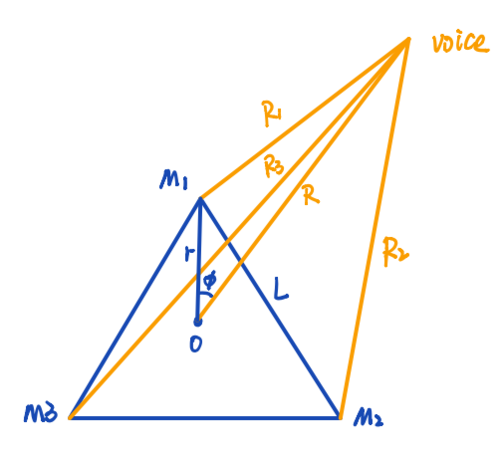
We can tell that the mathematical relationship are
$r={\frac {L}{\sqrt {3}}}$,
$R_{1}^{2}=R^{2}+r^{2}-2Rr\cos \phi$,
$R_{2}^{2}=R^{2}+r^{2}-2Rr\cos \left({\frac {2\pi }{3}}-\phi \right)$,
$R_{3}^{2}=R^{2}+r^{2}-2Rr\cos \left(\phi +{\frac {2\pi }{3}}\right)$.

And the distance difference:
$\Delta d_{12}=R_{2}-R_{1}=C\cdot \Delta t_{12}$,
$\Delta d_{13}=R_{3}-R_{1}=C\cdot \Delta t_{13}$,
$\Delta d_{23}=R_{3}-R_{2}=C\cdot \Delta t_{23}$.

So we can get
$\Delta d_{12}={\sqrt {R^{2}+r^{2}-2Rr\cos \left({\frac {2\pi }{3}}-\phi \right)}}-{\sqrt {R^{2}+r^{2}-2Rr\cos \phi }}=C\cdot \Delta t_{12}$,
$\Delta d_{13}={\sqrt {R^{2}+r^{2}-2Rr\cos \left(\phi +{\frac {2\pi }{3}}\right)}}-{\sqrt {R^{2}+r^{2}-2Rr\cos \phi }}=C\cdot \Delta t_{13}$,
$\Delta d_{23}={\sqrt {R^{2}+r^{2}-2Rr\cos \left(\phi +{\frac {2\pi }{3}}\right)}}-{\sqrt {R^{2}+r^{2}-2Rr\cos \left({\frac {2\pi }{3}}-\phi \right)}}=C\cdot \Delta t_{23}$.

If the $\phi$ is greater than $180^{\circ }$, we will take $360^{\circ }-\phi$ as the angle of the $\phi$, (i.e., the source is in the left plane divided by the line between the centre of gravity and M1) so that the angle of the $\phi$ stays between $0^{\circ }$-$180^{\circ }$.
In this case:
$R_{1}^{2}=R^{2}+r^{2}-2Rr\cos \phi$,
$R_{2}^{2}=R^{2}+r^{2}-2Rr\cos \left(\phi +{\frac {2\pi }{3}}\right)$,
$R_{3}^{2}=R^{2}+r^{2}-2Rr\cos \left({\frac {2\pi }{3}}-\phi \right)$.

The distance difference:
$\Delta d_{12}={\sqrt {R^{2}+r^{2}-2Rr\cos \left(\phi +{\frac {2\pi }{3}}\right)}}-{\sqrt {R^{2}+r^{2}-2Rr\cos \phi }}=C\cdot \Delta t_{12}$,
$\Delta d_{13}={\sqrt {R^{2}+r^{2}-2Rr\cos \left({\frac {2\pi }{3}}-\phi \right)}}-{\sqrt {R^{2}+r^{2}-2Rr\cos \phi }}=C\cdot \Delta t_{13}$,
$\Delta d_{23}={\sqrt {R^{2}+r^{2}-2Rr\cos \left({\frac {2\pi }{3}}-\phi \right)}}-{\sqrt {R^{2}+r^{2}-2Rr\cos \left(\phi +{\frac {2\pi }{3}}\right)}}=C\cdot \Delta t_{23}$.

Since we can measure and calculate the difference in distance between M2 and M3 (i.e. $\Delta d_{23}$), the first and second mathematical relationships are solved in terms of joint equations for $\Delta d_{23}>0$ and $\Delta d_{23}<0$, respectively. Then we can get $(R,\phi )$, and know the position of voice.

3-Dimensional

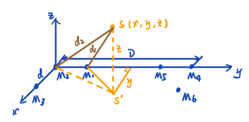
We can tell that the mathematical relationship are
$d_{2}^{2}=x^{2}+y^{2}+z^{2}$,
$d_{1}^{2}=z^{2}+(x-d)^{2}+y^{2}=z^{2}+x^{2}+d^{2}-2xd+y^{2}$,
$\Rightarrow d_{1}^{2}-d_{2}^{2}=d^{2}-2xd$,

${\sqrt {x^{2}+y^{2}+z^{2}}}=d_{2}={\frac {2d_{1}^{2}-2xd_{1}}{2(d_{2}-d_{1})}}$.
In the same way, we can get
$={\frac {1}{2(d_{2}-d_{1})}}(d_{1}^{2}+d_{2}^{2}-2xd_{1}-d_{1}^{2}+d_{2}^{2})$,
$={\frac {1}{2(d_{2}-d_{1})}}[(d_{2}-d_{1})^{2}-d_{1}^{2}+d_{2}^{2}]$,
$={\frac {1}{2C\cdot \Delta t_{21}}}[(C\cdot \Delta t_{21})^{2}+2xd_{1}-d_{1}^{2}]$.

So we can get the relationship between x and y,
$y=a_{1}x+b_{1}$,
which $a_{1}={\frac {\Delta t_{23}}{\Delta t_{21}}}$,
$b_{1}={\frac {(C^{2}\cdot \Delta t_{21}\cdot \Delta t_{23}+d^{2})(\Delta t_{21}-\Delta t_{23})}{2d\cdot \Delta t_{21}}}$.

$y=a_{2}x+b_{2}$,
which $a_{2}=-{\frac {\Delta t_{46}}{\Delta t_{45}}}$,
$b_{2}={\frac {\left[(C^{2}\cdot \Delta t_{45}\cdot \Delta t_{46}+d^{2})(\Delta t_{45}-\Delta t_{46})+2dD\Delta t_{45}\right]}{2d\cdot \Delta t_{45}}}$.

Using these two formulas $y=a_{1}x+b_{1}$
$y=a_{2}x+b_{2}$,
we can get $\Rightarrow {\hat {x}}={\frac {b_{2}-b_{1}}{a_{1}-a_{2}}}$
${\hat {y}}={\frac {a_{1}b_{2}-a_{2}b_{1}}{a_{1}-a_{2}}}$.

By inserting (x,y) into the distance difference formula, we can find the z value. Get the voice position S (x,y,z).

Cross-Correlation Function

Correlation function is a concept in signal analysis, representing the degree of correlation between two time series, that is, describing the degree of correlation between the values of signal x(t) and y(t) at any two different times t1 and t2. When describing the correlation between two different signals, the two signals can be random signals or they can be deterministic signals.

The correlation function can be used to calculate the arrival time difference of two sound signals, assuming that the signal received by microphone M1 is x(t), the signal received by microphone M2 is y(t)=Ax(t−t0), and the arrival time difference between sound waves arriving M1 and M2 is t0. Then the cross-correlation function of x(t) and y(t) is defined as

$\phi _{xy}(t)=\int _{-\infty }^{+\infty }x(\tau )y(t+\tau )d\tau =x(t)*y(-t)$.

Substituting the y(t) expression yields:

$\phi _{xy}(t)=\int _{-\infty }^{+\infty }x(\tau )x(t+\tau -t_{0})d\tau$,
${\text{when }}t=t_{0}{\text{, we can get the maximun of }}\phi _{xy}(t)=\int _{-\infty }^{+\infty }x(\tau )^{2}d\tau .$
According to $x(t)*y(-t)=X(\omega )Y^{*}(\omega )$,

$\phi _{xy}(t)=\int _{0}^{\pi }X(\omega )Y^{*}(\omega )e^{-j\omega t}d\omega$

Now $X(\omega )$ is the Fourier transform of $x(t)$，$Y(\omega )$ is the conjugate Fourier transform of $y(t)$. Some of $\omega$, the integral might correspond to the maximum value of $\phi _{xy}(t)$. Therefore, correlations can be quickly calculated by Fourier transforms and conjugate Fourier transforms.

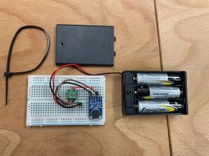
Experimental Setup

1. LeCroy - WaveSurfer - 64Xs - 600MHz Oscilloscope

LeCroy - WaveSurfer - 64Xs - 600MHz Oscilloscope

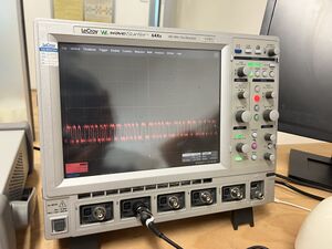
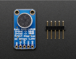
2. 3 integrated microphones (Adafruit AGC Electret Microphone Amplifier - MAX9814)

Adafruit AGC Electret Microphone Amplifier - MAX9814

3. Breadboard
4. Cables
5. Tape measure
6. 4.5V power supply

Complete built device

Measurements

1-Dimensional

1. One microphone was placed at 0cm as a reference and trigger, and the other microphone was placed 200cm away from it in a straight line. Both microphones were connected to an oscilloscope to obtain the waveform of the sound. (In the test experiments, we also set the straight line distance between the two microphones to 380cm, 100cm, etc.)

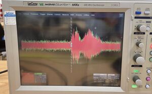
2. At 0, 50, 100, 150, and 200 cm points along the line between the two microphones, different sounds were produced, including clapping, and vocal sounds like "a", "hello", and "yes". The waveforms captured by the microphones were recorded on the oscilloscope.

'Hello' at 150.00cm

Sound source type: 'A'

3.In the extended experiment, we tried the same experiment as step 2 on the outside of the two microphones, i.e. -50, 250 cm.

4. MATLAB was used to analyze the recorded data. This involved calculating the time differences of arrival (TDOAs) of the sounds at the two microphones, from which the precise locations of the sounds were determined.

Data Processing

1-Dimensional

Data Collection

• Raw audio data were collected with two microphones, each recording saved as a '.dat' file.
• MATLAB was utilized for data importation and preliminary analysis.

Data Analysis Steps

1. Data Loading: Each microphone's data was loaded into MATLAB.
2. Distance Setting: A fixed distance of 'L' meters was maintained between both microphones.
3. Time and Amplitude Extraction: Time-stamped amplitude data were extracted from the audio files.
4. Amplitude Normalization: DC offset was mitigated by subtracting the mean amplitude from each signal.
5. Time Vector Adjustment: The time vector was recalibrated to start at zero, synchronizing the datasets.

Visualization

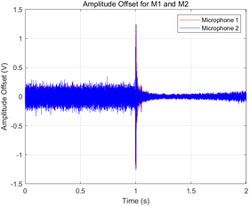
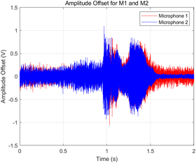
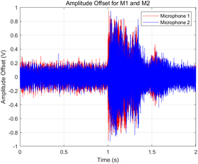
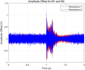
• Amplitude offsets for each microphone were plotted in a shared graph with distinct colors (red for Microphone 1 and blue for Microphone 2) to ensure clear differentiation.

Sound source type: Clap	Sound source type: 'Hello'
Sound source type: 'Yes'	Sound source type: 'A'

Cross-Correlation Analysis

• Temporal delays between signals were quantified through cross-correlation, pinpointing the sound's origination point relative to the microphones.

Sound Source Localization

• Employing the speed of sound (340 m/s), the source's location was computed based on the calculated time lag between the two signals.

Documentation and Output

• MATLAB commands were scripted to automate the processing steps, including normalization and cross-correlation plotting.
• The calculated time differences, delta distances, and source positions were output to the MATLAB console.

MATLAB code

1-Dimensional

 ch_0 = load('C1Trace00000.dat');
 ch_1 = load('C2Trace00000.dat'); % trigger, reference 
 L = 2; % dist btw 2 microphones
 time = ch_0(:, 1);
 dtime = ch_0(2, 1)- ch_0(1, 1);
 ch_0_ampl = ch_0(:, 2);
 ch_1_ampl = ch_1(:, 2);
 ch_0_ampl_mean = mean(ch_0_ampl);
 ch_1_ampl_mean = mean(ch_1_ampl);
 ch_0_ampl_offset = ch_0_ampl - ch_0_ampl_mean;
 ch_1_ampl_offset = ch_1_ampl - ch_1_ampl_mean;

 % Adjust time vector to start from 0
 time_adj = time - time(1);  % Subtract the first time value from all elements

 % Create a new figure window showing the first figure
 figure;
 plot(time_adj, ch_1_ampl_offset, 'r', time_adj, ch_0_ampl_offset, 'b');
 grid on;
 title('Amplitude Offset for M1 and M2');
 xlim([min(time_adj) max(time_adj)]);
 xlabel('Time (s)');
 ylabel('Amplitude Offset (V)');
 legend('Microphone 1', 'Microphone 2');

 [c, lag] = xcorr(ch_0_ampl_offset, ch_1_ampl_offset);
 % Create new figure window showing cross-correlation graphs
 figure;
 plot(dtime * lag, c);
 grid on;
 title('Cross-Correlation between M1 and M2');
 xlabel('Time Lag (s)');
 ylabel('Cross-Correlation');

 VS = 340; % speed of sound in ms^-1
 [val, index] = max(c);
 time_diff = dtime * lag(index);
 delta_x = time_diff * VS;
 x_pos = (L - delta_x) / 2;

 % Output calculation results
 disp(['Time Difference: ', num2str(time_diff), ' seconds']);
 disp(['Delta x: ', num2str(delta_x), ' meters']);
 disp(['Source Position: ', num2str(x_pos), ' meters']);

 % Compute normalized cross-correlation
 [c_norm, lag_norm] = xcorr(ch_0_ampl_offset, ch_1_ampl_offset, 'coeff');

 % Create a new graphics window to display the normalized cross-correlation graph
 figure;
 plot(dtime * lag_norm, c_norm);
 grid on;
 title('Normalized Cross-Correlation between M1 and M2');
 xlabel('Time Lag (s)');
 ylabel('Normalized Cross-Correlation');

 % Find the maximum value of the normalized cross-correlation and calculate the time difference
 [val_norm, index_norm] = max(c_norm);
 time_diff_norm = dtime * lag_norm(index_norm);

 % Output normalized calculation results
 disp(['Normalized Time Difference: ', num2str(time_diff_norm), ' seconds']);

Results

1-Dimensional

Results

Clap

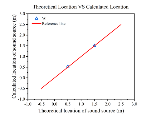
In our experiments, we first chose a single clap as the sound source. Multiple measurements were taken by clapping at locations between the two microphones, i.e., at 0, 50, 100, 150, and 200 cm, and the results are shown below.

Sound source type: Clap

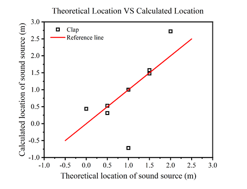
The figure shows the relationship between the theoretical position of the sound source and the calculated position. Since the horizontal coordinate is the theoretical position of the sound source, the vertical coordinate corresponding to the red straight line is the theoretical position of the sound source, so it is used as the reference line. The black square is the calculated sound source position.
Comparing the positions of the black square and the red line, it is found that the measurement error is larger at 0cm and 200cm (i.e., the positions of the two microphones), while the error is smaller at the position between the two microphones, and the closer to the midpoint of the two microphones, the closer to the theoretical position of the sound source is the calculated position of the sound source.
One of the points fell farther below the reference line when the theoretical position was 1.0 m. It is speculated that this may be due to an operational error during the measurement process.

Speech Commands: 'Hello', 'A', 'Yes'

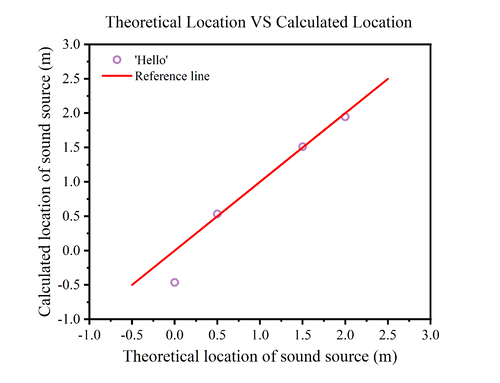
Due to the large error, we replaced the sound source with speech commands: 'Hello', 'A', 'Yes'. The experiment was repeated and the results obtained are shown in Fig.

Sound source type: 'Hello'

Sound source type: 'A'

In the left figure, we replace the sound source with the speech command: 'hello', and we can find that the calculated position at 0cm has a large error with the theoretical position, while the remaining points are almost on the reference line. In the right figure, the sound source is the speech command: 'A', and we can find that at 0.5m and 1.5m, the theoretical position is almost the same as the calculated position.
It can be noticed that when we change the sound source from clapping to speech command, the error decreases. However, there is still a higher probability of error when the sound source is at both ends, while in the middle of the two microphones, our measurements and code calculations are able to call a more accurate location of the sound source.

We also conducted several experiments when the sound source was 'yes', and in addition to measuring between the two microphones, we set the source at -50cm and 150cm for measurements.

Sound source type: 'Yes'

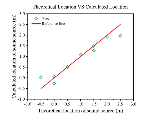
One measurement at 0cm and another at 150cm produced errors, so we conducted a second experiment at the same location and obtained better results at both points. This shows that the determination of the sound source position may be subject to errors due to some accidental factors. Since we used a mobile phone to play a speech command, it is possible that the orientation of the mobile phone may have an effect on the results.
Also, we notice that when we set the sound at -50, 150cm, the calculated positions are almost at the theoretical positions of 0cm and 200cm. This is in accordance with the theory that, assuming the sound is at -50cm, the difference in time for the sound to reach the two microphones is exactly the time difference caused by the distance between the two microphones.
Therefore, it is clear from the measurements that the device is not able to obtain the position of the sound source on the outside of the two microphones.

Aggregate Sound Source Positioning

We have summarised all the measurements on a single graph in order to check the performance of the sensor more clearly.

Relationship between theoretical and calculated positions when clapping as a sound source.

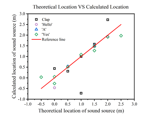
The figure shows the position measurements of the sensor for different sound sources at different locations. It can be noticed that the sensor performance is poorer and the error is larger when the sound is at the ends, and the closer the sound is to the midpoint of the two microphones, the smaller the measurement error is.
It is surmised that this may be because the closer the sound is to a particular microphone, the more easily chance variations can be sensitively reacted to this microphone. And when the sound is close to the middle, the resulting changes will be captured to the same extent by both microphones.
Clapping as a sound source may have a greater error than voice commands. This may be due to the fact that clapping sounds are more brief and sharp, which are less coherent and of short duration, making it difficult to extract precise temporal information from clapping sounds. Moreover, hand-clapping sounds contain a wide frequency range, including many high-frequency components, which may be subject to more attenuation and scattering during propagation, thus affecting measurement accuracy. On the contrary, voice commands have a long duration, a more regular and consistent acoustic pattern, a more concentrated frequency range, and a more stable acoustic signal.
In addition, there may be chance factors that affect the accuracy of the measurement, and multiple measurements may be required if accuracy is desired.

xcorr结果分析

看绝对系数大小，比较测量结果。下结论：xxx声音的展现的相关度最高

Error Analysis and Discussions

In the process of sound source localization using cross-correlation techniques in MATLAB, various factors can introduce significant errors. These include human-induced errors during operation and readings, as well as the intrinsic limitations of the `xcorr` function.

Human factors

• Manual Readings and Subjectivity:
  • It is often challenging to accurately determine the relative positions of two sound waves, leading to large errors. The direct reading of time differences (Δt) from the oscilloscope may therefore have limited reliability.
  • Comparative charts should be used to check for noticeable discrepancies in these readings.

• Optimal Parameter Settings:
  • Finding the most accurate setting for measurement parameters is crucial. Incorrect settings can lead to insufficient precision, significantly impacting the calculated results and the actual sound source location.
  • Time Division Settings: Larger time divisions may produce sharper peaks but decrease time precision, affecting overall location accuracy. Conversely, smaller divisions can increase precision but limit the measurable sound duration.
  • Voltage Division Settings: The ratio of the sound wave to the oscilloscope display scale must be optimally set to ensure that waveforms are neither too compressed nor too elongated, as both extremes can distort correlation accuracy.

Limitations of Cross-Correlation (xcorr)

• Sampling Frequency and Data Point Quantity:
  • Sampling Rate and Data Points: The accuracy of the time delay measured by the cross-correlation function (`xcorr`) is contingent upon the sampling rate and the number of data points.
    • If the sampling interval is too large or if the signal is not continuously recorded, the time delay derived may not be very precise.
    • Higher sampling rates can provide more detailed data and potentially more accurate delay estimates.

• Signal Characteristics and Noise:
  • Waveform Integrity and Noise: An incomplete waveform or significant noise within the signal can lead to erroneous interpretations by the cross-correlation algorithm.
    • Low-frequency oscillations or small amplitude variations can make it difficult for `xcorr` to accurately identify the delay corresponding to the peak correlation.
    • Ensuring high signal integrity and minimizing noise are crucial for reliable cross-correlation analysis.
  • Sound Signal Attenuation: The natural decay of the sound signal with distance may influence the code's ability to judge and compare waveforms accurately.
    • Sound intensity diminishes as it travels through the medium, which could lead to variations in the recorded waveforms at different distances.

• Boundary Effects and Window Size:
  • Effects of Signal Length and Window Size: The outcome of cross-correlation analysis is also influenced by the length of the signal and the size of the processing window.
    • Short signals or inappropriate window sizes can lead to misinterpretation of delays, affecting the overall results.
    • Adjusting the window size to adequately capture the dynamics of the signal without truncating important features is essential.

It is imperative to meticulously consider and, where possible, quantify each potential source of error. By doing so, the interpretation of data can be significantly enhanced, improving the reliability of the sound source localization methodology.

Logs

Build a link to record experiment log.

Sensor that recognizes specific sounds and steers toward the source

This is the name and link of the previous page. We adjusted the final project name displayed on the main page based on the final results and conditions.