Ultrasonic Doppler Speedometer

Objective

(1) Understand the principles of the ultrasonic Doppler effect and its application in speed measurement.

(2) Design and build an ultrasonic Doppler speedometer to measure the velocity of a moving object.

(3) Analyze experimental data and improve measurement accuracy.

Principle

The ultrasonic Doppler effect states that when ultrasonic waves encounter a moving target (such as a small car or fluid), the frequency of the reflected wave shifts. The frequency shift Δf is related to the velocity v of the target as follows:

$\mathrm{\Delta }f=\frac{2f_{0}v\cos \theta }{c}$

where c is the speed of sound in air; θ is the angle between the wave propagation direction and the target's motion.

Methods and Results

Raw Data

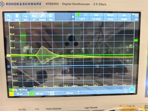
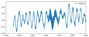
First, we display the waveform shown on the oscilloscope. The following image shows the transmitted and received waveforms.（Take a distance of 10cm as an example）

Waveform Analysis and Fourier Transform

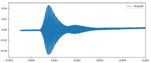
Next, we analyze the waveforms using Python. The transmitted waveform is a square wave, while the received waveform is more complex, resembling a sinusoidal waveform that is a sum of many sine waves.

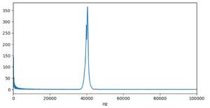
We perform a Fourier Transform on the received waveform to analyze its frequency content. The Fourier transform result is as follows:

From this plot, we observe that the received waveform contains a significant amount of low-frequency noise, which we need to filter out.

This low-frequency noise is common in laboratory environments and can originate from several sources:

• Power line interference: 50 Hz or 60 Hz noise from AC mains power is often present in lab equipment and cables.
• Electronic device vibrations: Fans, transformers, or other nearby equipment can produce low-frequency mechanical vibrations.
• Human activity and footsteps: Physical movement near the setup may introduce low-frequency noise through the table or sensor supports.
• Ambient acoustic noise: Conversations or nearby machinery can contribute sound energy at low frequencies.

To ensure accurate signal interpretation, especially in ultrasonic experiments, these noise components must be filtered out before further analysis.

Digital Filtering

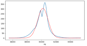
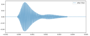
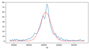
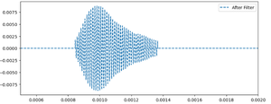
To remove the background noise, we apply a digital filter. After filtering, the frequency spectrum and waveform are significantly improved, showing much less noise. We also fit the filtered frequency spectrum using a Gaussian (normal distribution) curve to estimate the dominant frequency component, which results in a mean frequency of 40012.77 Hz. The filtered results are shown below:

As shown, the noise is greatly reduced after filtering, making the waveform more suitable for experimental analysis.

Measurement of Sound Velocity

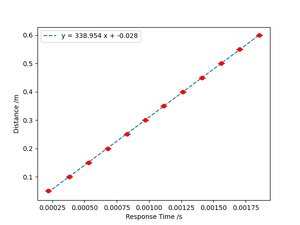
We measured waveforms from the detected sensor with various sensor-sensor distances. Considering the time difference between the transmitting sensor's waveform and the detecting sensor's waveform as the response time that the ultrasonic wave spreads this distance, we plotted the response time versus distance curve as follows:

In this plot, we can find the slope in the fitted curve around 338.95 m/s, which is close to the theoretical air sound velocity (343 m/s), with an error of around 1.18%.

It is worth noting that the speed of sound in air is affected by several environmental factors:

• Temperature: Sound velocity increases with temperature. For example, at 20 °C, the velocity is approximately 343 m/s, but at 0 °C it drops to about 331 m/s.
• Humidity: Higher humidity levels can increase the sound speed because water vapor is less dense than dry air.
• Air pressure and altitude: At constant temperature, changes in pressure have minimal effect, but at high altitudes where both pressure and temperature drop, sound speed decreases.
• Gas composition: Sound speed also depends on the medium's composition. For instance, sound travels faster in helium than in air.

These factors may contribute to slight deviations between the measured and theoretical values.

Doppler Effect Measurement of Sound Velocity

In this section, we explore another method to measure the speed of sound using the Doppler effect. We move the ultrasonic receiver at a constant speed of 10 cm/s and analyze the frequency shift due to the relative motion between the transmitter and receiver.

Raw Waveform Observation

The waveform collected during receiver motion is shown below（Take a distance of 10cm/s as an example）:

As we can see, the raw waveform contains significant noise — even more than the previous static measurement. This is mainly due to mechanical vibrations and irregular contact with the metal rail on which the ultrasonic receiver was moving. Metal surfaces can introduce:

• High-frequency jitter from mechanical contact irregularities,
• Low-frequency rumble due to structural vibrations,
• Reflections and scattering, especially at non-uniform metal junctions.

Filtering and Signal Recovery

To isolate the useful frequency information, we apply digital filtering similar to the previous section. The filtered waveform and frequency spectrum are shown below:

The signal is now cleaner, and a clear frequency shift can be observed.

Doppler Effect Analysis

The Doppler effect equation for sound waves when the receiver is moving towards the stationary transmitter is:

$f^{\prime }=f(1+\frac{v}{c})$

Where:

• $f^{\prime }$ is the observed frequency,
• $f$ is the transmitted (original) frequency,
• $v$ is the velocity of the receiver (toward the source),
• $c$ is the speed of sound in air.

We rearrange the equation to solve for $c$:

$c=\frac{vf}{f^{\prime }-f}$

We compute the measured sound velocity using the detected frequency shift. A comparison with the actual speed (10 cm/s) is shown below:

Measured Frequency (Hz)	Original Frequency (Hz)	Velocity (cm/s)	Calculated Sound Speed (m/s)	Error (%)
...	...	10	...	...

Appendix

Python Code for Signal Processing and Sound Speed Estimation

Below is the Python code used to read oscilloscope data, calculate time-of-flight (ToF), estimate distances, and plot the comparison between actual and estimated distances.

<syntaxhighlight lang="python"> import pandas as pd import numpy as np import matplotlib.pyplot as plt

def process_ultrasound_csv(file_path, encoding='utf-8', sound_speed=343):

   df = pd.read_csv(file_path, usecols=[0, 1, 2], encoding=encoding, skip_blank_lines=True)
   df.columns = ['时间', '接收信号', '输出信号']

   time = df['时间'].values
   tx = df['输出信号'].values
   rx = df['接收信号'].values

   tx_threshold = 0.5 * (np.max(tx) - np.min(tx)) + np.min(tx)
   tx_index = np.argmax(tx > tx_threshold)
   tx_time = time[tx_index]

   rx_index = np.argmax(rx)
   rx_time = time[rx_index]

   tof = rx_time - tx_time
   distance_estimated = tof * sound_speed

   return {
       'tx_time': tx_time,
       'rx_time': rx_time,
       'tof': tof,
       'distance_estimated': distance_estimated
   }

</syntaxhighlight>

<syntaxhighlight lang="python">

1. 多文件批量处理函数

def process_multiple_ultrasound_files(file_paths_dict, encoding='utf-8', sound_speed=343):

   results = {}
   for distance_cm, file_path in file_paths_dict.items():
       result = process_ultrasound_csv(file_path, encoding=encoding, sound_speed=sound_speed)
       results[distance_cm] = result
   return results

</syntaxhighlight>

<syntaxhighlight lang="python">

1. 绘图函数：实际距离 vs 估计距离

def plot_estimated_vs_actual(results_dict):

   actual = []
   estimated = []
   for distance_cm, res in results_dict.items():
       actual.append(distance_cm / 100)
       estimated.append(res['distance_estimated'])

   coeffs = np.polyfit(actual, estimated, deg=1)
   fitted = np.polyval(coeffs, actual)

   plt.figure(figsize=(6, 6))
   plt.scatter(actual, estimated, color='dodgerblue', label='Estimated distance')
   plt.plot(actual, fitted, 'r-', label=f'fitting: y = {coeffs[0]:.3f}x + {coeffs[1]:.3f}')
   plt.xlabel('Actual distance (m)')
   plt.ylabel('Estimated distance (m)')
   plt.title('Actual distance vs Estimated distance')
   plt.legend()
   plt.grid(True)
   plt.axis('equal')
   plt.tight_layout()
   plt.show()

</syntaxhighlight>

<syntaxhighlight lang="python">

1. 调用部分

file_paths = {

   cm: fr"C:\Users\70905\Downloads\WFM\WFM\WFM_{cm}cm_01.CSV"
   for cm in range(5, 65, 5)

} all_results = process_multiple_ultrasound_files(file_paths)

1. 打印结果

for distance_cm, res in all_results.items():

   print(f"{distance_cm}cm 结果：ToF = {res['tof']:.6f}s, 估计距离 = {res['distance_estimated']:.3f}m")

plot_estimated_vs_actual(all_results) </syntaxhighlight>

Python Code for Signal Processing

<syntaxhighlight lang="python"> import numpy as np import math import matplotlib.pyplot as plt import pandas as pd from scipy.optimize import curve_fit from scipy.stats import norm

file_dir = f'C:\\Users\\70905\\Documents\\WeChat Files\\wxid_msmjcahnii2f22\\FileStorage\\File\\2025-04\\WFM\\WFM\\WFM_10cm_01.CSV'

1. file_dir = f'E:\\Studying\\24-25 Semester2\\Physics of Sensors\\WFM'

df = pd.read_csv(file_dir)

signal = df['C1 in V'].values T = df['in s'].values

plt.figure(figsize=(8, 4)) plt.plot(T, signal) plt.xlabel('s') plt.show() dt = T[2] - T[1] n = len(signal) N_pad = 50*n signal_padded = np.zeros(N_pad) signal_padded[:n] = signal

fft_vals = np.fft.fft(signal_padded) freqs = np.fft.fftfreq(N_pad, dt)

pos_mask = freqs >= 0 freqs = freqs[pos_mask] fft_vals = fft_vals[pos_mask] amplitudes = np.abs(fft_vals) max_index = np.argmax(amplitudes[5000:]) dominant_freq = freqs[max_index + 5000] print(f"{dominant_freq} Hz")

plt.figure(figsize=(8, 4)) plt.plot(freqs,amplitudes) plt.xlim(0,1e5) plt.xlabel('Hz') plt.show()

1. 定义高斯函数：用于拟合

def gauss(x, amp, mean, sigma):

   return amp * np.exp(-(x - mean)**2 / (2 * sigma**2))

cutoff_freq = 5000 filter_mask1 = np.abs(freqs) < dominant_freq + cutoff_freq filter_mask2 = np.abs(freqs) > dominant_freq - cutoff_freq filter_mask = filter_mask1 * filter_mask2 filtered_fft = fft_vals * filter_mask filtered_fft2 = np.abs(filtered_fft.copy()) idx_sorted = np.argsort(filtered_fft2) second_idx = idx_sorted[-1]

1. print(freqs[second_idx])

1. 对滤波后的数据进行拟合

freq_filtered = freqs[filter_mask] # 滤波后的频率 amplitudes_filtered = np.abs(filtered_fft[filter_mask]) # 滤波后的幅度

1. 初始猜测值：幅度最大值、均值（主频）、标准差（根据宽度估计）

initial_guess = [np.max(amplitudes_filtered), dominant_freq, np.std(freq_filtered)]

1. 拟合高斯曲线

params, covariance = curve_fit(gauss, freq_filtered, amplitudes_filtered, p0=initial_guess)

1. 提取拟合参数

amp_fit, mean_fit, sigma_fit = params

1. 打印拟合结果

print(f"拟合的高斯分布参数：") print(f"幅度：{amp_fit}") print(f"均值（中心频率）：{mean_fit:.2f} Hz") print(f"标准差：{sigma_fit:.2f} Hz")

1. 生成拟合曲线

x_fit = np.linspace(np.min(freq_filtered), np.max(freq_filtered), 1000) y_fit = gauss(x_fit, *params)

plt.figure(figsize=(8, 4)) plt.plot(freqs[filter_mask], np.abs(filtered_fft[filter_mask])) plt.plot(x_fit, y_fit, label="高斯拟合曲线", linestyle="--", color="red") plt.xlabel('Hz') plt.show()

filtered_signal = np.fft.ifft(filtered_fft) filtered_signal = np.real(filtered_signal)[:n]

plt.figure(figsize=(10, 4)) plt.plot(T,signal, label='Orignial') plt.xlim(-0.001, 0.005) plt.legend() plt.show()

T2 = np.linspace(T[0],T[-1],len(filtered_signal)) B = [] s = 15e-4 Tr = 0 for i in range(len(T2)):

   if abs(filtered_signal[i]) >= s :
       B.append(1)
       if Tr == 0:
           Tr += 1
   else :
       B.append(0)

filtered_signal = filtered_signal*np.array(B)

plt.figure(figsize=(10, 4)) plt.plot(T2*math.pi,filtered_signal, label='After Filter', linestyle='--') plt.xlim(-0.001, 0.005) plt.legend() plt.show() </syntaxhighlight>